hvega-0.9.0.0: README.md
# hvega
[](https://vega.github.io/vega-lite/)
Create [Vega-Lite](https://vega.github.io/vega-lite/) visualizations in
Haskell. It targets version 4.12 of the Vega-Lite specification. Note that
the module does not include a viewer for these visualizations (which are
JSON files), but does provide several helper functions, such as
[toHtmlFile](https://hackage.haskell.org/package/hvega/docs/Graphics-Vega-VegaLite.html#v:toHtmlFile),
which create HTML that can be viewed
with a browser to display the visualization. Other approaches include
automatic display in IHaskell notebooks - with the
[ihaskell-vega](https://hackage.haskell.org/package/ihaskell-hvega)
package - or use of external viewers such as
[Vega View](https://hackage.haskell.org/package/vega-view) and
[Vega-Desktop](https://github.com/vega/vega-desktop).
It started off being a copy on an early version (2.2.1) of the
[Elm Vega library](http://package.elm-lang.org/packages/gicentre/elm-vega/2.2.1/VegaLite),
which is released under a BSD3 license by Jo Wood of the giCentre at the
City University of London.
This code is released under the BSD3 license.
## Examples
### Cars
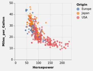
The [Vega-Lite example gallery](https://vega.github.io/vega-lite/examples/) contain
a number of visualizations of the `cars.json` dataset, which has a number of
columns to display, such as "Horsepower", "Miles_per_Gallon", and "Origin". The
following code will create a visualization that plots the efficiency of the
cars (the "mpg") as a function of its Horsepower, and color-code by the
origin of the car:
```Haskell
let cars = dataFromUrl "https://vega.github.io/vega-datasets/data/cars.json" []
enc = encoding
. position X [ PName "Horsepower", PmType Quantitative ]
. position Y [ PName "Miles_per_Gallon", PmType Quantitative ]
. color [ MName "Origin", MmType Nominal ]
bkg = background "rgba(0, 0, 0, 0.05)"
in toVegaLite [ bkg, cars, mark Circle [], enc [] ]
```
When the JSON is viewed with a Vega-Lite aware viewer, the resultant plot is
### Betelgeuse
In late 2019 and early 2020 the
[star Betelgeuse](https://en.wikipedia.org/wiki/Betelgeuse) - a member of the
[constellation Orion](https://en.wikipedia.org/wiki/Orion_(constellation)) -
dimmed enough that you could see it. Betelgeuse is a member of the class of
Red Supergiant stars, which are massive enough that they will go supernova
at some point, and so there was
[some speculation](https://en.wikipedia.org/wiki/Betelgeuse#2019%E2%80%932020_fading)
that we could see a "naked-eye" supernova (even though the current models
suggest that Betelgeuse has about 100,000 more years to go before this happens).
This interest lead to a lot of observations added to the
[American Association of Variable Star Observers](https://www.aavso.org/)
database, which we are going to look at below. This example is rather-more
involved than the case one, since it involves data filtering and creation,
multiple plots, faceting, and interactive selection.
```Haskell
let titleStr = "Betelegeuse's magnitude measurements, collated by AAVSO"
w = width 600
h = height 150
pos1Opts fld ttl = [PName fld, PmType Quantitative, PAxis [AxTitle ttl]]
x1Opts = pos1Opts "days" "Days since January 1, 2020"
y1Opts = pos1Opts "magnitude" "Magnitude" ++ [PSort [Descending], yRange]
yRange = PScale [SDomain (DNumbers [-1, 3])]
filtOpts = [MName "filterName", MmType Nominal]
filtEnc = color (MLegend [ LTitle "Filter", LTitleFontSize 16, LLabelFontSize 14 ] : filtOpts)
. shape filtOpts
circle = mark Point [ MOpacity 0.5, MFilled False ]
encOverview = encoding
. position X x1Opts
. position Y y1Opts
. filtEnc
selName = "brush"
pos2Opts fld = [PName fld, PmType Quantitative, PAxis [AxNoTitle],
PScale [SDomain (DSelectionField selName fld)]]
x2Opts = pos2Opts "days"
y2Opts = pos2Opts "magnitude" ++ [PSort [Descending]]
encDetail = encoding
. position X x2Opts
. position Y y2Opts
. filtEnc
xlim = (Number (-220), Number 100)
ylim = (Number (-0.5), Number 2.5)
overview = asSpec [ w
, h
, encOverview []
, selection
. select selName Interval [ Encodings [ChX, ChY]
, SInitInterval (Just xlim) (Just ylim)
]
$ []
, circle
]
detailPlot = asSpec [ w
, h
, encDetail []
, circle
]
headerOpts = [ HLabelFontSize 16
, HLabelAlign AlignRight
, HLabelAnchor AEnd
, HLabelPadding (-24)
, HNoTitle
, HLabelExpr "'Filter: ' + datum.label"
]
details = asSpec [ columns 1
, facetFlow [ FName "filterName"
, FmType Nominal
, FHeader headerOpts
]
, spacing 10
, specification detailPlot
]
in toVegaLite [ title titleStr [ TFontSize 18 ]
, dataFromUrl "https://raw.githubusercontent.com/DougBurke/hvega/master/hvega/data/betelgeuse-2020-03-19.json" []
, transform
. filter (FExpr "datum.filterName[0] === 'V'")
. filter (FExpr "datum.magnitude < 4")
. calculateAs "datum.jd - 2458849.0" "days"
$ []
, vConcat [overview, details]
, configure
. configuration (Axis [ TitleFontWeight Normal, TitleFontSize 16, LabelFontSize 14 ])
$ []
]
```
This can be viewed as
- an [interactive version](https://vega.github.io/editor/#/url/vega-lite/N4KABGBEAuBOCGA7AzgMwPawLaQFxgG1wIxhJUBLAG2gFNY8oATeaAVywDpKb6A5eFloEADAF0wAXmlgA5ADVZkAL4AaYhDI86DfJBbsuWeAHNEFdk1pgAPGAAsK9SVKR4yRvvgBPD6qgAxvBUAWxUrLSeBhycAFZMYAC0YABM9gCsAByZ9gCcnCIqxGLOgeiIlCaMoC5uAB4UHvg1LlDQFlS0AGLl0ADqtBQmABbQnoiYxlSQpbXhAEa0VD2I0ADKFABekfgAjPazJDAd3b0b24y7AGwaYMrEasRe0PDVt5BssNN6o9AADshcAB6IEIADunBMFmGbHmbGQ9ACvVoq04SKwQIAIug2CYAEKfADWtCBwwAbrQTPAgcZkDpSRSqUCDNTFnQqCZaPDaIkUiI+YkRABmRK7fKxZDlSAPUqQMlIxBBMb4IguFq1YaDEbKsC7dIiQ4QSDGWCE6qQdB-eABCzeRgiTjpfwwbx-HZQP7oCirGZQHidJiMVDBBGPVpQMEUJjQYaMK4iA23I0IzoBdpS5pJo7zWDw2OZ8O1b0Wc11RgEXl8-y7BMlKB2lWCx3+FKOsRhwtGlFIpjekxNQiQMvOu0lLO1aCu92Qb06MnBaWd+7hju1bvoXuIKoFwuQJFUTBvTtGyhLQN6bT8QSRQ2tF1u8boLDehe3uaUlHn0jju8LJYrdYtndfY3zvdpoE6TwumoHQZh-CcTgA85gJuY87h-Vc72QYZ4AfZpyAoM9PEvWABCEX172nCZn0QBdMNqMsd07AiiL0FhfDgtDKM8ABHNgkHA1gKApTjj3qRpzXAyC9ExHxkDAZBvQCawACkkH42BvF1Ft+UKZdC3oo4G2-LjTyoL9jVMcxLBveCoGQIJpNcJgn3gb1y1FfwhXbUDk0wHV9FoBzPz7UTmMnPCoD4gSLCEkTfKgeAGgHMgpOnABZKyLDYKwiiXLN9IgTD1SOZA3QCI9d01IZRkufVQMs01zUta1bXtZs2inTxPVnCj-VoL9gyoUMGsjaN8zAeNE2Y9dN23EyxP3Q8mLEsyLJIsjbLQo0Iqop8X2mBKjU6TlEC-EquL-ZYziAy4DjshCIOnaDeAYI6jjSpDbr2VDtsKgyEsgbDcPdLRCPM4iYKvcjnV2x8aLowHGIW0zwYs9i-Ae+zHNB-RXPc-C1qiOSKJTWg0woDMoBzPMVEM8NuL0aLVli9p4qx8SUuOJ7GEQMIqH+ldAeMi7dyJvRjDMbLcveoGcfNFzjAJ1xxagSXrJym97KWcn00QTwaewunZclWAAqsYKztC2W4aZ-iWZeNmtu2znJJOXn+cF1ovaKgrbz3dAqA4FBLn94NlJ1UWTzRyHXs2sK701eArF0FHdyugBBRVhmWqBPwThmroAUTqP5U8gWQXp0fBZDAABqMBoi4K6C9-eBFioAAFZO5sYXl7su9v-xui4fsBtKPaoKhAczqghn1vRYBqsYMIa22oGog7F29-2ytardLhEW59LHI0ABIHM1YxPF+AFgSBRl4EhaFYU4SmgUv2hjAfyl4ESOe6AP3sHESU+tZQTxWjAWgdQAp4loOyD83JZDyXVtLawQh3CfC-iiaAyB-D7nCHQBI8wtIZwzvINYAB5BO5AR7AUyDKJ4FsAhLz+HrTwAAJdAYIwA4XknA9knIkHyRzMvRAQV5LziXgNfw8x3ADTAOURurB4BgAIREYhpDyFULAAAClvoCEEYJjGcHgPAMkkpOCYBMECAAlJwMAABNHECkc5hASCGdAYADzoEJGAVgvDoD-EMUCaAkYgn0DRE+IEbIljzHQNAfxZ1AnBPvlCGMr90SkgoH8P4xIYnwLiQkhxABJRJYJ3D+KnmAGM1gECckUYgBS6AbTBDAEIXsqiAm1IUi8M2ijUCpF0pwaUyggA)
- as a PNG:

## Documentation
A tutorial is provided as part of the module: it is based, as is
so much of the module, on the
[Elm Vega walk through](https://github.com/gicentre/elm-vegalite/tree/master/docs/walkthrough).
The tutorial
is [available on hackage](https://hackage.haskell.org/package/hvega/docs/Graphics-Vega-Tutorials-VegaLite.html) - and includes the plot outputs -
and the plots it creates are also available by importing the
`Graphics.Vega.Tutorials.VegaLite` module.
The
[Vega-Lite Example Gallery](https://vega.github.io/vega-lite/examples/) has
been converted to IHaskell notebooks in the
[notebooks directory](https://github.com/DougBurke/hvega/tree/master/notebooks).
Start with the
[overview notebook](https://github.com/DougBurke/hvega/blob/master/notebooks/VegaLiteGallery.ipynb),
which describes the set up, and then the individual
sections have their own notebooks (with names of
`VegaLiteGallery-<section>.ipynb`.
Unfortunately the plots created by VegaEmbed **do not always appear**
in the notebook when viewed with either GitHub's viewer or
[ipynb viewer](http://nbviewer.jupyter.org/github/DougBurke/hvega/blob/master/notebooks/VegaLiteGallery.ipynb),
but things seem better when using Jupyter Lab (rather than
notebook) to create the notebooks (since Vega is natively
supported in this environment). However, the native support is
for Vega-Lite version 1, and so many of the more-recent
capabilities are either ignored or cause the visualization to
fail.
The notebooks have been re-created
using Jupyter Lab (thanks to Tweag I/O's
[JupyterWith environment](https://www.tweag.io/posts/2019-02-28-jupyter-with.html)), which should make the plots appear on GitHub (you may need
to reload the notebooks as I find they don't display on the
first try).
## Differences to Elm Vega
Elm Vega has changed significantly since I started `hvega`, and no-longer
exposes data types directly but uses functions instead: for example,
rather than `PName`, it uses a function like `pName`. It is an open
question whether `hvega` will make the same switch. Over time
the naming of certain operations or data types has diverged between
`hevga` and Elm Vega.
One of the more-obvious changes is that the output of `toVegaLite`
is a separate type from the input values - that is `VegaLite`
and `VLSpec` - since it makes it easier to display the output of
`hvega` in `IHaskell`. The JSON specification is retrieved from
this type with `fromVL`. The `0.5.0.0` release adds some more
type safety (restricting the functions that can be applied
to `encoding` and `transform` for instance).