gulcii-0.3: doc/encoding.md
# Lambda calculus encodings
## Notation
Backslash is used for lambda:
* easier to type
* familiar from Haskell
Neighbouring lambdas can be combined with one backslash:
\a b s z . a s (b s z)
Corresponds to:
λa. λb. λs. λz. a s (b s z)
## Church and Scott encodings
* encode data as lambda terms
* continuation passing style
* Church folds vs Scott case analysis
## Continuation passing style
* the datum is a black box that knows itself
* the datum is passed functions that it calls with its deconstruction
* the datum has one argument per constructor
* each continuation has one argument per constructor argument
## Simple types
Church and Scott encoding coincide for simple types.
## Bool
Haskell:
data Bool
= False
| True
Church, Scott:
true = \t f . t
false = \t f . f
and = \a b . a b a
or = \a b . a a b
not = \a . a false true
The datum "true" takes two arguments, and returns the first, which (by
convention) denotes the value True.
## Pair
Haskell:
data Pair a b
= Pair a b
Church, Scott:
pair = \a b p . p a b
fst = \p . p (\a b . a)
snd = \p . p (\a b . b)
The datum "pair x y" takes one argument, which is a function of two arguments,
and passes it the stored values of "x" and "y".
## Maybe
Haskell:
data Maybe a
= Nothing
| Just a
Church, Scott:
nothing = \n j . n
just = \a n j . j a
maybe = \n j m . m n j
## Either
Haskell:
data Either a b
= Left a
| Right b
Church, Scott:
left = \a l r . l a
right = \b l r . r b
either = \l r e . e l r
## Recursive types
* Church and Scott encoding differ for recursive types.
* Church encoding uses folds.
The deconstruction continuation threads throughout
the structure.
* Scott encoding is similar to case analysis.
The deconstruction continuation
unwraps one layer of constructors only.
## Natural numbers
Haskell:
data Nat
= Zero
| Succ Nat
Church:
zero = \s z . z
succ = \n s z . s (n s z)
Scott:
zero = \s z . z
succ = \n s z . s n
## Nat examples
Haskell:
Zero, Succ Zero, Succ(Succ Zero), Succ(Succ(Succ Zero))
Church, applying the same "s" "n" times at once:
\s z . z
\s z . s z
\s z . s (s z)
\s z . s (s (s z))
Scott, applying different "s" "n" times separately:
\s z . z
\s z . s (\s z . z)
\s z . s (\s z . s (\s z . z))
\s z . s (\s z . s (\s z . s (\s z . z)))
## Church Nat succ
zero = \s z . z
succ = \n s z . s (n s z)
succ zero
= {- definition of succ -}
(\n s z . s (n s z)) zero
= {- beta -}
\s z . s (zero s z)
= {- definition of zero -}
\s z . s ((\s z . z) s z)
= {- beta -}
\s z . s ((\z . z) z)
= {- beta -}
\s z . s z
= {- definition of one -}
one
## Scott Nat succ
zero = \s z . z
succ = \n s z . s n
succ zero
= {- definition of succ -}
(\n s z . s n) zero
= {- beta -}
\s z . s zero
= {- definition of zero -}
\s z . s (\s z . z)
= {- definition of one -}
one
## Nat arithmetic
Church:
add = \m n . m succ n
mul = \m n . m (add n) zero
exp = \m n . n m
Scott, open terms with `letrec`:
add = \m n . m (\p . succ (add p n)) n
mul = \m n . m (\p . add n (mul p n)) zero
exp = \m n . n (\p . mul m (exp m p)) one
Scott, closed terms with `fix`:
add = fix (\add . \m n . m (\p . succ (add p n)) n)
mul = fix (\mul . \m n . m (\p . add n (mul p n)) zero)
exp = fix (\exp . \m n . n (\p . mul m (exp m p)) one)
## Fixed point combinator
Semantics:
fix f = f (fix f)
Implementation:
\f . (\x . f (x x)) (\x . f (x x))
What it computes:
* The unique least fixed point under the definedness order.
* Allows recursive functions to be defined as closed terms.
## Nat predecessor
Church (courtesy Wikipedia):
pred = \n f x . n (\g h . h (g f)) (\u . x) (\v . v)
Scott:
pred = \n . n (\p . p) zero
## Nat conversion
Church arithmetic is more concise (and doesn't need `fix`).
Scott predecessor is comprehensible.
Mix and match?
churchToScott = \n . n scottSucc scottZero
scottToChurch = \n . n
(\p . churchSucc (scottToChurch p))
churchZero
scottToChurch = fix (\scottToChurch . \n . n
(\p . churchSucc (scottToChurch p))
churchZero)
## Nat subtract and equality
Church:
sub = \m n . n pred m
Scott:
sub = \m n . m
(\p . n (\q . sub p q) m)
zero
equal = \m n . m
(\p . n (\q . equal p q) false)
(n (\q . false) true)
Unwrap a layer of constructor from each number and recurse.
There is a different `equal` for booleans:
equalBool = \a b . a b (not b)
## List
Haskell:
data List a
= Nil
| Cons a (List a)
Church:
nil = \c n . n
cons = \x xs c n . c x (xs c n)
Scott:
nil = \c n . n
cons = \x xs c n . c x xs
## List operations
Church, Scott:
isnil = \l . l (\x xs . false) true
head = \l . l (\x xs . x) error
Church (`tail` courtesy Wikipedia):
length = \l . l (\x xs . succ xs) zero
tail = \l c n . l
(\x xs g . g x (xs c)) (\xs . n) (\x xs . xs)
Scott:
length = \l . l (\x xs . succ (length xs)) zero
tail = \l . l (\x xs . xs) nil
## More Scott functions
compose = \f g x . f (g x)
fold = \f e l . l (\x xs . f x (fold f e xs)) e
sum = fold add zero
ands = fold and true
ors = fold or false
map = \f . fold (compose cons f) nil
all = \f . compose ands (map f)
any = \f . compose ors (map f)
take = \n l. n(\p. l (\x xs. cons x (take p xs))nil)nil
drop = \n l. n(\p. l (\x xs. drop p xs) nil) l
iterate = \f x . cons x (iterate f (f x))
# How to perform lambda calculus
## How to perform lambda calculus
* single step graph reduction
* visualisation of current state
* sonification of changes in state
* open terms vs closed terms
## Graph reduction
data Term
= Free String
| Reference Integer
| Bound -- de Bruijn index 0
| Scope Term -- see Lambdascope paper
| Lambda Strategy Term
| Apply Term Term
reduce
:: Definitions -- Map String Term
-> References -- Map Integer Term
-> Term
-> Maybe (References, Term)
## Three kinds of Lambda
* strict (syntax inspired by Haskell's -XBangPatterns):
(\v ! s) t
t is fully reduced before substitution into s.
* copy:
(\v ? s) t
t is substituted for each occurrence of v in s.
* lazy:
(\v . s) t
a new `Reference` is created for t, and substituted into s.
`reduce` reduces *inside* the `References` until it is irreducible, at which
point the `Reference` is replaced with the `Term` it refers to.
## Visualisation
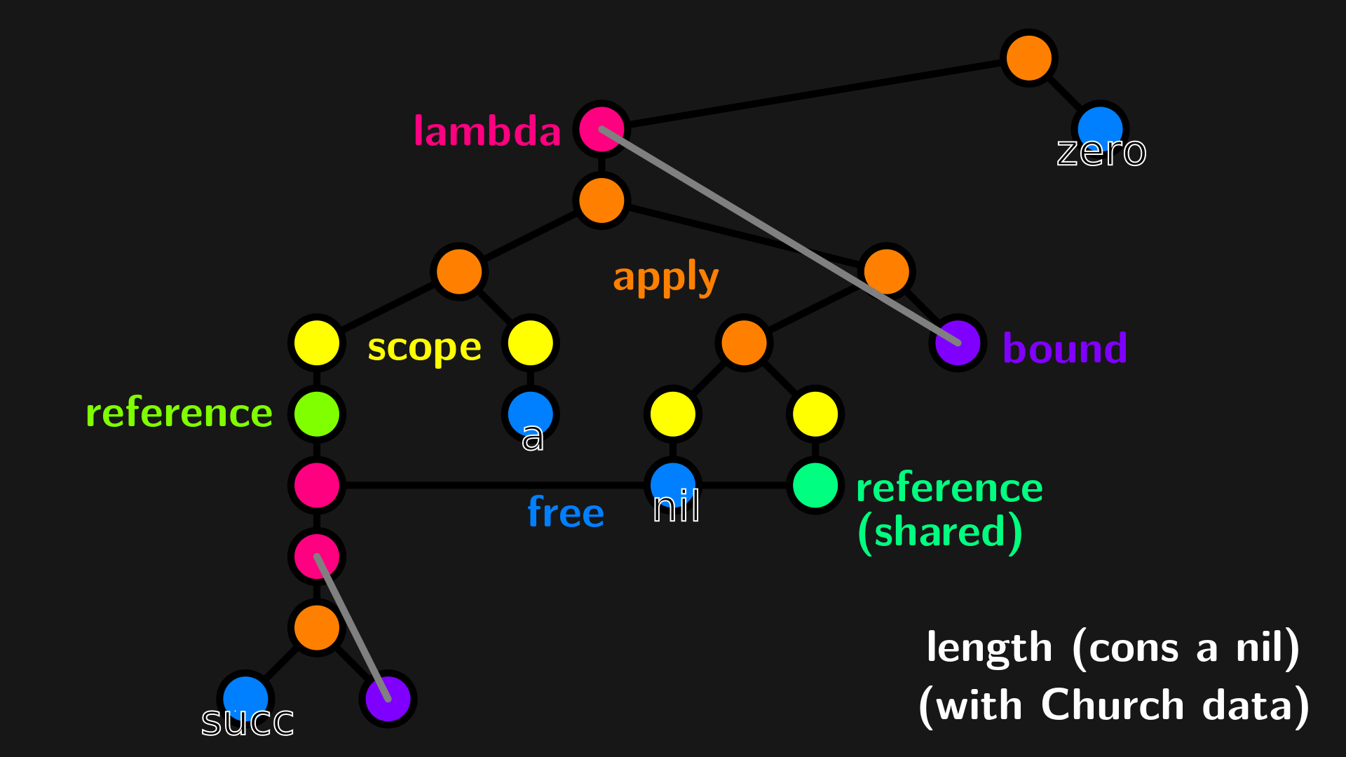{width=100%}\
## Sonification
* count number of nodes of each type
* statistics are forwarded to a Pure-data patch
* changes in each count control a harmonic (one for each type of node) in a
simple phase modulation synth
## Open terms
* free variables looked up on demand from environment
* allows definitions to be changed at runtime
* easier to write
## Drawbacks of open terms
* no sharing
subterms can be evaluated many times due to duplication
* exponential work (worst case)
* exponential space (worst case)
## Fixed points
* closed terms with fixed point combinators
* allows evaluation to be shared
* sharing can be vital for efficiency
# Future work
## Better Evaluator
* current evaluator is still somewhat ad-hoc and doesn't preserve sharing
* previous evaluator even had correctness bugs
* switch to using Lambdascope (or similar) as a library?
## Auto Fix
Automatically translating open terms to use fixed point combinators:
* recursive functions can use `fix`
* mutually recursive functions can use `fix` combined with tuples
many = some `orElse` none
some = one `andThen` many
becomes:
manysome = fix (\p -> pair
(snd p `orElse` none)
(one `andThen` fst p) )
many = fst manysome
some = snd manysome
## Magic It
* refer to previously evaluated terms
* including the currently evaluating term
* without restarting evaluation
Haskell example (`ghci-8.0.1`):
> 3
3
> it + 5
8
> it * 2
16
## Further Performances / Project Ideas
* "An infinite deal of nothing", a variety of non-terminating loops each with
their own intrinsic computational rhythm.
* Implement in untyped lambda calculus an interpreter for a known
Turing-complete tape mutation based language and run some simple programs
in it.
Illustrates Turing-completeness of untyped lambda calculus, albeit slowly.
# EOF
## EOF
Thanks!
Questions?
https://mathr.co.uk
mailto:claude@mathr.co.uk
https://hackage.haskell.org/package/gulcii
https://code.mathr.co.uk/gulcii