CPL-0.2.0: TUTORIAL.md
# CPL Tutorial
## Introduction
CPL (Categorical Programming Language) is a programming language designed based on concepts from category theory. In CPL, what are typically referred to as “data types” and “functions” in conventional programming languages are instead treated as “objects” and “morphisms” (or “arrows”) in category theory.
|Set Theory|Functional Programming|CPL|
|-|-|-|
|Set|Data Type|Object|
|Mapping|Function|Morphism|
### Key Features of CPL
- **Category-theoretic data type definition**: All data types are defined using category theory concepts, specifically F,G-dialgebras—a generalization of adjunctions and F-(co)algebras
- **Type safety**: A robust type system grounded in category theory principles
- **Functional programming**: Only total functions are supported, ensuring pure computation without side effects
- **Duality**: Symmetric design using both `left object` (initial structure) and `right object` (terminal structure)
### Prerequisite Knowledge
For optimal understanding, familiarity with the following:
- Basic programming concepts
- Experience with functional programming languages like Haskell (though not mandatory)
No prior knowledge of category theory is required. Through this tutorial, you'll learn both CPL usage and fundamental category theory concepts.
### What You'll Learn from This Tutorial
- Basic CPL operations: REPL usage, data type definition, and function definition
- Fundamental category theory concepts: Terminal/initial objects, products/coproducts, exponential objects, etc.
- The distinction between `left objects` and `right objects`, and the concept of duality in category theory
- Practical programming examples: Natural numbers, lists, infinite lists, etc.
## Table of Contents
- [Introduction](#introduction)
- [Basic Commands](#basic-commands)
- [Initial Screen Display](#initial-screen-display)
- [Defining Terminal Objects](#defining-terminal-objects)
- [Defining Cartesian Products](#defining-cartesian-products)
- [Defining Exponential Objects](#defining-exponential-objects)
- [Defining the Natural Numbers Object](#defining-the-natural-numbers-object)
- [Defining Coproducts](#defining-coproducts)
- [Displaying Types](#displaying-types)
- [Composing Morphisms and Identity Morphisms](#composing-morphisms-and-identity-morphisms)
- [Assigning Names to Expressions](#assigning-names-to-expressions)
- [Computation](#computation)
- [List Types](#list-types)
- [Infinite Lists](#infinite-lists)
- [Category Theory Background: Left vs. Right](#category-theory-background-left-vs.-right)
- [Summary](#summary)
- [References](#references)
## Basic Commands
The CPL REPL (Read-Eval-Print Loop) supports the following commands. This section provides only an overview, with detailed usage examples to be learned through practical application.
- **`edit`**: Enters multi-line editing mode. Use this for defining data types. End editing mode by entering semicolon (`;`)
- **`show <expression>`**: Displays the type (domain and codomain) of an morphism (function)
- **`show object <functor>`**: Displays detailed information about an object (data type)
- **`show function <function>`**: Displays the type of a factorizer (higher-order function) or user-defined function
- **`let <name> = <expression>`**: Defines an morphism by assigning it a name
- **`let <name>(<arguments>) = <expression>`**: Defines an morphism with parameters
- **`simp <expression>`**: Simplifies (computes) the given expression
- **`simp full <expression>`**: Fully simplifies the expression (use when `simp` alone cannot complete simplification)
- **`it`**: Refers to the result from the previous computation
- **`load <filename>`**: Loads definitions from a file
- **`help`**: Displays help information
- **`exit`**: Exits the CPL environment
## Initial Screen
Upon startup, the interface appears as follows:
```
Categorical Programming Language (Haskell version)
version 0.1.0
Type help for help
cpl>
```
## Defining the Terminal Object
CPL has no built-in data types, and all data types must be explicitly defined.
Since every operation requires the **terminal object**—corresponding to the unit type in other functional programming languages—we begin by defining this fundamental concept.
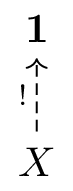
In category theory, a **terminal object** `1` is defined as “an object such that for every object `X`, there is exactly one morphism from `X` to `1`.” It serves as an “endpoint” representing an object with no information (or containing only one value). The unique morphism is written as `!`.
Visually, this corresponds to the following situation:
Correspondences to programming concepts:
- Haskell's `()` type (unit type)
- `void` or `unit` types in other languages
- The concept of “a type containing exactly one value”
Now, let's define the terminal object in CPL. Using the `edit` command, enter multi-line editing mode, input your data type definition, and exit multi-line editing mode by entering semicolon `;`.
```
cpl> edit
| right object 1 with !
| end object;
right object 1 defined
```
The output “`right object 1 defined`” confirms that the terminal object `1` has been successfully defined.
Detailed information about a defined object can be viewed using `show object`.
```
cpl> show object 1
right object 1
- natural transformations:
- factorizer:
----------
!: *a -> 1
- equations:
(RFEQ): 1=!
(RCEQ): g=!
- unconditioned: yes
- productive: ()
```
When object 1 is defined, a special morphism `!` is also defined from any object to the terminal object.
The `show` command can also be used to display the morphism's type (domain and codomain). Here, `*a` is a variable representing an object, so this represents an morphism from any object to the terminal object 1.
```
cpl> show !
!
: *a -> 1
```
## Defining the Product
Next, we'll define the **product**. The product combines two objects into a single object.
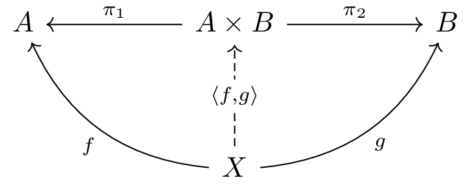
In category theory, the product `A × B` (`prod(a,b)` in CPL) is defined as “an object that preserves the information of both objects `A` and `B`.” It satisfies the following properties:
- Existence of projection morphisms `π₁: A × B → A` and `π₂: A × B → B`
- For any object `X` with morphisms `f: X → A` and `g: X → B` to `A` and `B` respectively, there exists a unique morphism `⟨f,g⟩: X → A × B` such that `π₁ ∘ ⟨f,g⟩ = f` and `π₂ ∘ ⟨f,g⟩ = g` (this kind of property is referred to as the **universal property**).
Visually represented as a diagram:
Correspondences with programming concepts:
- Haskell's `(a, b)` type (tuple)
- Pairs or structures in other languages
- The concept of “a type that combines two values”
Now, let's define the product in CPL:
```
cpl> edit
| right object prod(a,b) with pair is
| pi1: prod -> a
| pi2: prod -> b
| end object;
right object prod(+,+) defined
```
(Note in the definition of `pi1` and `pi2` that the object `prod` we're defining now lacks arguments. The mearning is “Among all `x` equipped with `x -> a` and `x -> b`, we define the most general `x` as `prod(a,b)`,” but resuing the name `prod` instead of introducing a new name `x`)
Unlike in the case of terminal objects, the product `prod(a,b)` is an object that takes parameters, and the resulting definition displays as `prod(+,+)`. The `+` indicates covariance, and we can see that `prod` takes two arguments and is covariant with respect to both arguments. Use `show object` to display detailed information.
```
cpl> show object prod
right object prod(+,+)
- natural transformations:
pi1: prod(*a,*b) -> *a
pi2: prod(*a,*b) -> *b
- factorizer:
f0: *a -> *b f1: *a -> *c
------------------------------
pair(f0,f1): *a -> prod(*b,*c)
- equations:
(REQ1): pi1.pair(f0,f1)=f0
(REQ2): pi2.pair(f0,f1)=f1
(RFEQ): prod(f0,f1)=pair(f0.pi1,f1.pi2)
(RCEQ): pi1.g=f0 & pi2.g=f1 => g=pair(f0,f1)
- unconditioned: yes
- productive: (yes,yes)
```
Unlike terminal objects, in the case of products, both projection morphisms `pi1` and `pi2` are defined simultaneously (you can also check their types using the `show` command).
Additionally, a function (factorizer) `pair` is also defined, which constructs `pair(f,g): a -> prod(b,c)` from `f: a -> b` and `g: a -> c`. The morphism previously written as `⟨f,g⟩` is now written as `pair(f,g)` in this definition of products in CPL. The factorizer `pair` itself is not an morphism and cannot be displayed using `show`; instead, use `show function` to display its type.
```
cpl> show function pair
f0: *a -> *b f1: *a -> *c
------------------------------
pair(f0,f1): *a -> prod(*b,*c)
```
Furthermore, while `prod` maps objects `a` and `b` to the object `prod(a,b)`, it also maps morphisms `f: a -> c` and `g: b -> d` to `prod(a,b) -> prod(b,d)`. In category theory, a **functor** maps objects to objects and morphisms between objects to morphisms between mapped objects. Using `show function prod`, you can verify the type of `prod`'s action on morphisms.
```
cpl> show function prod
f0: *a -> *c f1: *b -> *d
---------------------------------------
prod(f0,f1): prod(*a,*b) -> prod(*c,*d)
```
Furthermore, examining `equations` reveals that the following four equalities hold. Here, the `.` notation represents **morphism composition**, meaning `g.f` means “first apply `f`, then apply `g`” (corresponding to the mathematical notation `g ∘ f`).
- (REQ1): `pi1.pair(f0,f1)=f0`
- (As stated earlier as a property of the product)
- (REQ2): `pi2.pair(f0,f1)=f1`
- (Same as above)
- (RFEQ): `prod(f0,f1)=pair(f0.pi1,f1.pi2)`
- (Definition of `prod` in terms of `pair` and `pi1`, `pi2`)
- (RCEQ): `pi1.g=f0 & pi2.g=f1 => g=pair(f0,f1)`
- (If `g` satisfies the same conditions as `pair(f0,f1)`, then `g=pair(f0,f1)`, i.e., `pair(f0,f1)` is unique)
## Definition of Exponential Object
Next, we define the **exponential object**, which is a structure for treating functions as values.
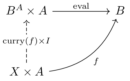
The exponential object `Bᴬ` (denoted as `exp(a,b)` in CPL) represents “the object that encodes all morphisms from `A` to `B`.” It possesses the following properties:
- An evaluation morphism `eval: Bᴬ × A → B` exists, allowing functions to be applied to values
- (While we call it `eval` here, in functional programming contexts, `apply` would be a more natural name)
- For any morphism `f: X × A → B`, there exists a unique curried morphism `curry(f): X → Bᴬ` satisfying `eval ∘ (curry(f) × I) = f`
- (Here, `I: A → A` represents the identity morphism, and `×` denotes the product morphism operation)
Visualized as a diagram, it appears as follows:
**Why Is the Exponential Object Called a “Function Space”?** Let's consider this concretely in the context of the category of sets.
- **Bᴬ is the set of all functions from A to B** — In the category of sets, the exponential object `Bᴬ` is the set `{f | f: A → B}` of functions itself.
- **eval represents function application** — `eval(f, a) = f(a)`. In other words, it performs the operation of “taking a pair of a function `f` and its argument `a`, and returning the result of applying `f` to `a`.”
- **curry represents argument separation** — For `f: X × A → B`, `curry(f)(x)` returns the function `a ↦ f(x, a)`. In other words, currying transforms a two-argument function into a one-argument function that returns another function — this is precisely the operation of converting a function into a function that returns functions.
- **Universality characterizes the function space** — The commutativity of the diagram above — the property that “functions from `X × A → B` are in one-to-one correspondence with functions from `X → Bᴬ`” — is what uniquely characterizes `Bᴬ` as a function space. This correspondence is exactly the relationship between currying and function application in programming.
Correspondences with programming concepts:
- Haskell's `a -> b` type (function type)
- Currying and function application
- The concept of “treating functions as first-class values”
A category equipped with the terminal object, product objects, and exponential objects is called a Cartesian Closed Category, which forms the theoretical foundation for lambda calculus and functional programming.
Now, let's define the exponential object in CPL:
```
cpl> edit
| right object exp(a,b) with curry is
| eval: prod(exp,a) -> b
| end object;
right object exp(-,+) defined
```
We can display detailed information using `show object`:
```
cpl> show object exp
right object exp(-,+)
- natural transformations:
eval: prod(exp(*a,*b),*a) -> *b
- factorizer:
f0: prod(*a,*b) -> *c
---------------------------
curry(f0): *a -> exp(*b,*c)
- equations:
(REQ1): eval.prod(curry(f0),I)=f0
(RFEQ): exp(f0,f1)=curry(f1.eval.prod(I,f0))
(RCEQ): eval.prod(g,I)=f0 => g=curry(f0)
- unconditioned: yes
- productive: (no,no)
```
We can see that `eval` for function application, `curry` for currying, and the conditions for an exponential object in category theory are all defined.
Let's examine how the functor `exp` operates on morphisms using `show function`:
```
cpl> show function exp
f0: *c -> *a f1: *b -> *d
------------------------------------
exp(f0,f1): exp(*a,*b) -> exp(*c,*d)
```
Note the directionality of the argument morphisms, and how the parameters of `exp` change from domain to codomain in the result:
- `f0` is a morphism from `*c` to `*a`, but the parameter changes direction from `*a` to `*c` in the result
- `f1` is a morphism from `*b` to `*d`, and the direction of the parameter is the same, from `*b` to `*d`
This indicates that `exp` is a contravariant functor with respect to the first argument and a covariant functor with respect to the second argument. The notation `exp(-,+)` used during definition and in `show object exp` is a concise representation of this property.
## Definition of the Natural Numbers Object
A **natural numbers object** is an inductively defined structure characterized by the number 0 and the successor function.
The natural numbers object `ℕ` is uniquely characterized by the following elements:
- Zero `0: 1 → ℕ` (the initial value)
- Successor function `s: ℕ → ℕ` (also denoted as `succ`, the function that increments by 1)
- For any object `X` and morphisms `z: 1 → X` and `f: X → X`, there exists a unique morphism `pr(z,f): ℕ → X` defined recursively such that `pr(z,f) ∘ 0 = z` and `pr(z,f) ∘ s = f ∘ pr(z,f)`
This `pr` operation corresponds to **mathematical induction** and serves as the fundamental method for defining functions over the natural numbers.
Visualized graphically, this structure appears as follows:
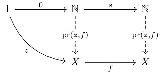
Please note the direction of the arrows. Whereas in the terminal objects, products, and exponential objects we have handled so far, there existed a unique morphism with that object as its *codomain*, in the case of the natural numbers object, conversely, there exists a unique morphism with that object as its *domain*.
Correspondences to programming concepts:
- The definition of natural numbers according to Peano's axioms
- Equivalent to Haskell data types such as:
```haskell
data Nat = Zero | Succ Nat
```
- Recursive computations (folding)
Now, let's define the natural numbers object in CPL. While we have previously defined objects as `right object`s when there exists a unique morphism with that object as their *codomain*, we now define the natural numbers object as `left object` as there exists a unique morphism with that object as their *domain*:
```
cpl> edit
| left object nat with pr is
| 0: 1 -> nat
| s: nat -> nat
| end object;
left object nat defined
```
To display the defined information, use `show object nat`:
```
cpl> show object nat
left object nat
- natural transformations:
0: 1 -> nat
s: nat -> nat
- factorizer:
f0: 1 -> *a f1: *a -> *a
-------------------------
pr(f0,f1): nat -> *a
- equations:
(LEQ1): pr(f0,f1).0=f0
(LEQ2): pr(f0,f1).s=f1.pr(f0,f1)
(LFEQ): nat=pr(0,s)
(LCEQ): g.0=f0 & g.s=f1.g => g=pr(f0,f1)
- unconditioned: no
- productive: ()
```
Here, `0` and `s` represent the zero and successor functions respectively, while `pr` corresponds to mathematical induction, along with the conditions they must satisfy.
## Defining the Coproduct
**The coproduct** is a structure representing “either-or,” serving as the dual concept to the direct product.
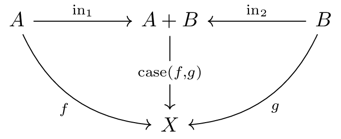
The coproduct `A + B` (denoted as `coprod(a,b)` in CPL) is an object that can hold one of two values, either from object `A` or `B`:
- It has two injection morphisms `in₁: A → A + B` and `in₂: B → A + B` (which “inject” values into the coproduct)
- For any objects `X` and morphisms `f: A → X` and `g: B → X`, there exists a unique morphism `case(f,g): A + B → X` that combines them case-by-case, satisfying `case(f,g) ∘ in₁ = f` and `case(f,g) ∘ in₂ = g`
This is the dual concept of the product, obtained by “reversing the arrow,” and serves as a good example of symmetry in category theory.
Visualized graphically, it appears as follows: (Compare with the product diagram to verify that morphisms are reversed):
Correspondences to programming concepts:
- Haskell's `Either a b` type
- `variant` types or other languages' `union` types with tags
- Branching logic using pattern matching
Now let's define the coproduct in CPL:
```
cpl> edit
| left object coprod(a,b) with case is
| in1: a -> coprod
| in2: b -> coprod
| end object;
left object coprod(+,+) defined
```
```
cpl> show object coprod
left object coprod(+,+)
- natural transformations:
in1: *a -> coprod(*a,*b)
in2: *b -> coprod(*a,*b)
- factorizer:
f0: *b -> *a f1: *c -> *a
--------------------------------
case(f0,f1): coprod(*b,*c) -> *a
- equations:
(LEQ1): case(f0,f1).in1=f0
(LEQ2): case(f0,f1).in2=f1
(LFEQ): coprod(f0,f1)=case(in1.f0,in2.f1)
(LCEQ): g.in1=f0 & g.in2=f1 => g=case(f0,f1)
- unconditioned: yes
- productive: (no,no)
```
## Displaying Type Information
The `show` command can be used to display the types of morphisms (their domains and codomains).
```
cpl> show pair(pi2,eval)
pair(pi2,eval)
: prod(exp(*a,*b),*a) -> prod(*a,*b)
```
Here, `*a` and `*b` are variable ranging over objects, and the morphism actually denotes families of morphisms with varying types (domains and codomains). When these families satisfy certain conditions, they are called **natural transformations**, which correspond to **polymorphic functions** in typical functional programming languages.
In the above example, `pair(pi2,eval)` is an morphism that works for any objects `*a` and `*b`, and can be viewed as a natural transformation from the functor `F(*a,*b) = prod(exp(*a,*b),*a)` to the functor `G(*a,*b) = prod(*a,*b)`.
## Morphism Composition and Identity Morphisms
The `.` symbol appearing in the equations above refers to fundamental operations on morphisms, which we will now review.
### Morphism Composition
`.` represents **morphism composition**. Given morphisms `f: A → B` and `g: B → C`, the composed morphism `g.f: A → C` is the morphism that “first applies `f`, then applies `g`”. This corresponds to the mathematical notation `g ∘ f` (the Unicode symbol `∘` is also usable in CPL).
For example, we can represent natural numbers by composing the successor function `s: nat → nat` with the zero `0: 1 → nat`:
```
cpl> show s.0
s.0
: 1 -> nat
cpl> show s.s.s.0
s.s.s.0
: 1 -> nat
```
`s.s.s.0` represents the “morphism obtained by composing `s` (successor function) three times with `0`”, which corresponds to the natural number **3**. Similarly, `s.s.0` represents **2**, and `s.0` represents **1**.
### Identity Morphisms
The **identity morphism** `I` is the “do-nothing” morphism, with `I: A → A` existing for any object `A`:
```
cpl> show I
I
: *a -> *a
```
An identity morphism satisfies `f.I = f` and `I.f = f`. While it may seem trivial at first glance, we frequently use it in conjunction with functors to “transform only one of the components while leaving the other unchanged”:
```
cpl> show prod(s, I)
prod(s,I)
: prod(nat,*a) -> prod(nat,*a)
```
Here, `prod(s, I)` represents the morphism that “applies `s` to the first component of the product while leaving the second component unchanged.”
## Naming Expressions
The `let` command allows us to assign names to morphisms, enabling subsequent reference by name. This enables us to construct complex morphisms step by step.
As our first example, let's define the natural number addition `add: prod(nat, nat) → nat`. This would be a function typically written as follows:
```haskell
add 0 y = y
add (x + 1) y = add x y + 1
```
In CPL, we express this using primitive recursion `pr` combined with currying `curry`. Let's break it down step by step.
1. **Strategy**: We want to use primitive recursion `pr` on the first argument, but `pr(f0, f1): nat → X` can only define unary morphisms. Therefore, we **curry** the second argument by encapsulating it within the exponential object.
2. **Curried addition `add'`**:
- `add': nat → exp(nat, nat)` — An morphism that takes a natural number `n` and returns a “function that adds `n`”
- This can be defined in the form of `pr(f0, f1)`
3. **`f0 = curry(pi2)` (zero case)**:
- `add'(0)` returns “the function that adds 0” = the identity function
- `pi2: prod(1, nat) → nat` is an morphism that extracts the second component of a product, which here functions as “discarding the first component (the unique value of the terminal object) while returning the second argument unchanged”
- `curry(pi2): 1 → exp(nat, nat)` serves as the base case for the zero case
4. **`f1 = curry(s.eval)` (successor case)**:
- `add'(n+1)` returns “a function that applies `s` to the result of `add'(n)`”
- `eval: prod(exp(nat,nat), nat) → nat` represents function application
- `s.eval: prod(exp(nat,nat), nat) → nat` performs “function application followed by taking the successor”
- `curry(s.eval): exp(nat,nat) → exp(nat,nat)` represents the recursive step
5. **Uncurrying**: Revert `add' = pr(curry(pi2), curry(s.eval))` back to `eval` and `prod`:
- `prod(add', I): prod(nat, nat) → prod(exp(nat,nat), nat)` — Applies `add'` to the first argument
- `eval.prod(add', I): prod(nat, nat) → nat` — Applies the resulting function to the second argument
Putting it all together:
```
cpl> let add=eval.prod(pr(curry(pi2), curry(s.eval)), I)
add : prod(nat,nat) -> nat defined
```
In the `let` construct, we can also define morphisms with parameters.
```
cpl> let uncurry(f) = eval . prod(f, I)
f: *a -> exp(*b,*c)
-----------------------------
uncurry(f): prod(*a,*b) -> *c
```
## Computation
In CPL, computation is performed through simplification of morphism expressions using the `simp` command. Let's simplify an morphism using our previously defined addition function `add`.
```
cpl> simp add.pair(s.s.0, s.0)
s.s.s.0
: 1 -> nat
```
The result `s.s.s.0` represents applying the successor function `s` three times, corresponding to the natural number 3. This demonstrates the calculation 2 + 1 = 3.
Similar to addition, let's define and compute multiplication and factorial.
**Multiplication** `mult: prod(nat, nat) → nat` can be defined using the same pattern as addition (currying + primitive recursion + uncurrying):
```
cpl> let mult=eval.prod(pr(curry(0.!), curry(add.pair(eval, pi2))), I)
mult : prod(nat,nat) -> nat
```
The differences from `add` lie only in the zero case and the recursive step:
- **Zero case** `curry(0.!)` — `0 × y = 0` (`0.!` is an morphism that returns zero regardless of input)
- **Successor case** `curry(add.pair(eval, pi2))` — `(n+1) × y = n × y + y` (adds the recursive result `eval` to `y` itself `pi2`)
**Factorial** `fact: nat → nat` uses a slightly different approach. It carries the state of `prod(nat, nat)` (a pair of accumulator and counter) using `pr`:
```
cpl> let fact=pi1.pr(pair(s.0,0), pair(mult.pair(s.pi2,pi1), s.pi2))
fact : nat -> nat defined
```
- **Initial value** `pair(s.0, 0)` — `(1, 0)`, i.e. “0! = 1, counter = 0”
- **Recursive step** `pair(mult.pair(s.pi2, pi1), s.pi2)` — computes `(acc, k)` to `((k+1) × acc, k+1)`
- **Final result** `pi1` extracts the accumulator value (the factorial result)
Let's compute it:
```
cpl> simp fact.s.s.s.s.0
s.s.s.s.s.s.s.s.s.s.s.s.s.s.s.s.s.s.s.s.s.s.s.s.0
: 1 -> nat
```
Since `s` has been applied 24 times, we obtain the correct result 4! = 24.
## List Type
Next, we'll define a **list type**—a data structure that's very similar to natural numbers but slightly more complex.
Lists, like natural numbers, have an inductive structure, but they differ in that lists are parameterized by their element type:
- Empty list `nil: 1 → list(a)`
- Element prepend `cons: a × list(a) → list(a)` (adds an element to the front)
- Fold `prl(z,f): list(a) → b` for recursively processing lists
Visualized graphically:
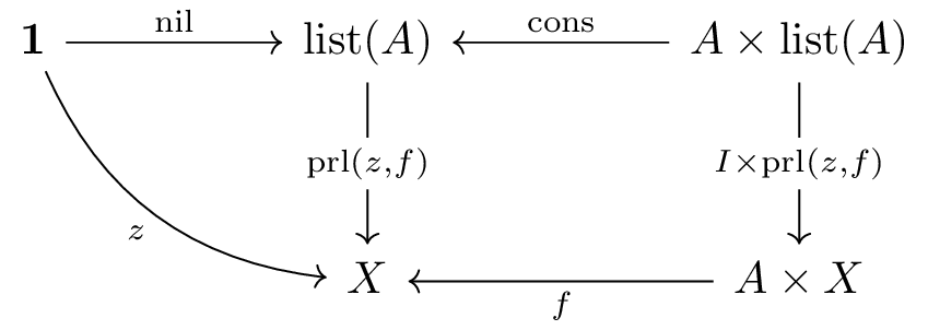
This represents a classic example of an **inductive data type** that describes finite structures.
Correspondence with programming:
- Haskell's `[a]` type (lists)
- Folding using `foldr`
Now let's define lists in CPL:
```
cpl> edit
| left object list(p) with prl is
| nil: 1 -> list
| cons: prod(p,list) -> list
| end object;
left object list(+) defined
```
```
cpl> show function list
f0: *a -> *b
------------------------------
list(f0): list(*a) -> list(*b)
cpl> show object list
left object list(+)
- natural transformations:
nil: 1 -> list(*a)
cons: prod(*a,list(*a)) -> list(*a)
- factorizer:
f0: 1 -> *a f1: prod(*b,*a) -> *a
----------------------------------
prl(f0,f1): list(*b) -> *a
- equations:
(LEQ1): prl(f0,f1).nil=f0
(LEQ2): prl(f0,f1).cons=f1.prod(I,prl(f0,f1))
(LFEQ): list(f0)=prl(nil,cons.prod(f0,I))
(LCEQ): g.nil=f0 & g.cons=f1.prod(I,g) => g=prl(f0,f1)
- unconditioned: no
- productive: (no)
```
The list is also a parameterized object, that is, a functor. Let's examine its action on morphisms. In functional programming, this action of the list functor on morphisms is often referred to as `map`.
```
cpl> show function list
f0: *a -> *b
------------------------------
list(f0): list(*a) -> list(*b)
```
Next, let's express some familiar functions using the list type.
Concatenation (`append`):
```
cpl> let append = eval.prod(prl(curry(pi2), curry(cons.pair(pi1.pi1, eval.pair(pi2.pi1, pi2)))), I)
append : prod(list(*a),list(*a)) -> list(*a) defined
```
Reversal (`reverse`):
```
cpl> let reverse=prl(nil, append.pair(pi2, cons.pair(pi1, nil.!)))
reverse : list(*a) -> list(*a) defined
```
`head` / `tail`:
```
cpl> let hd = prl(in2, in1.pi1)
hd : list(*a) -> coprod(*a,1) defined
cpl> let tl = coprod(pi2,I).prl(in2, in1.prod(I, case(cons,nil)))
tl : list(*a) -> coprod(list(*a),1) defined
```
We've chosen `hd` / `tl` here because we want to use these names when working with infinite lists later. In CPL, since only total functions exist and no partial functions are allowed, the codomain is a coproduct with `1` (equivalent to the `Maybe` or `Option` types in other languages).
For convenience, we've also defined versions that lift the domain to the coproduct with `1`, allowing us to apply `head` / `tail` to the results of these operations again.
```
cpl> let hdp=case(hd,in2)
hdp : coprod(list(*a),1) -> coprod(*a,1) defined
cpl> let tlp = case(tl, in2)
tlp : coprod(list(*a),1) -> coprod(list(*a),1) defined
```
Sequential numbers `[n-1, n-2, ..., 1, 0]`:
```
cpl> let seq = pi2.pr(pair(0,nil), pair(s.pi1, cons))
seq : nat -> list(nat) defined
```
Now, let's perform some computations.
Some calculations require `simp full` instead of just `simp` to proceed with reduction.
```
cpl> simp seq.s.s.s.0
cons.pair(s.pi1,cons).pair(s.pi1,cons).pair(0,nil)
: 1 -> list(nat)
cpl> simp full seq.s.s.s.0
cons.pair(s.s.0,cons.pair(s.0,cons.pair(0,nil)))
: 1 -> list(nat)
```
While `simp` alone stops at an intermediate form, `simp full` completes the full reduction. The result `cons.pair(s.s.0,cons.pair(s.0,cons.pair(0,nil)))` represents list notation in CPL. In other languages, this corresponds to the list `[2, 1, 0]`:
| CPL Representation | Meaning |
|---|---|
| `nil` | `[]` (Empty list) |
| `cons.pair(x, xs)` | `x : xs` (Prepend `x` to the beginning of `xs`) |
| `cons.pair(s.s.0, cons.pair(s.0, cons.pair(0, nil)))` | `[2, 1, 0]` |
Let's examine the results of computing with other functions as well:
```
cpl> simp hdp.tl.seq.s.s.s.0
in1.s.0
: 1 -> coprod(nat,*a)
```
Since `seq.s.s.s.0` equals `[2, 1, 0]`, applying `tl` to remove the head yields `[1, 0]`, and then applying `hdp` to get the head results in `in1.s.0` (which equals `Just 1`).
```
cpl> simp full append.pair(seq.s.s.0, seq.s.s.s.0)
cons.pair(s.0,cons.pair(0,cons.pair(s.s.0,cons.pair(s.0,cons.pair(0,nil)))))
: 1 -> list(nat)
cpl> simp full reverse.it
cons.pair(0,cons.pair(s.0,cons.pair(s.s.0,cons.pair(0,cons.pair(s.0,nil.!)))))
: 1 -> list(nat)
```
`append.pair(seq.s.s.0, seq.s.s.s.0)` concatenates `[1, 0]` and `[2, 1, 0]` to form `[1, 0, 2, 1, 0]`, while `reverse.it` reverses this to produce `[0, 1, 2, 0, 1]`.
In the final example `simp full reverse.it`, we use `it` to reference the result of the previous computation (`append.pair(seq.s.s.0, seq.s.s.s.0)`). `it` is a useful feature that automatically stores the result of the immediately preceding `simp` command.
### Differences Between `simp` and `simp full`
CPL provides two reduction commands:
- **`simp`**: Performs basic reduction. Fast but may stop prematurely
- **`simp full`**: Performs more thorough reduction. Use when a completely reduced form is required
## Infinite Lists
In addition to finite data types like natural numbers and lists, we can also define data types for **infinite lists**.
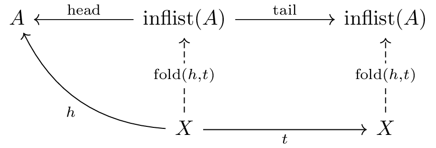
Unlike finite lists, infinite lists are defined as a `right object`. This is an example of a **coinductive data type**:
- `head: inflist(a) → a` (extracts the head element)
- `tail: inflist(a) → inflist(a)` (obtains the remaining infinite list)
- `fold(h,t): x → inflist(a)` allows unfolding the infinite list (note that while named `fold`, in modern functional programming conventions this would more appropriately be called `unfold`)
While finite lists operate by “building up and then consuming,” infinite lists have the contrasting structure of “unfolding from state.”
Visualized graphically:
Corresponding to programming concepts:
- Haskell's lazy evaluation-based infinite lists
- Streams and iterators
- Generation via `unfold`
Now let's define an infinite list in CPL.
```
cpl> edit
| right object inflist(a) with fold is
| head: inflist -> a
| tail: inflist -> inflist
| end object;
right object inflist(+) defined
```
```
cpl> show object inflist
right object inflist(+)
- natural transformations:
head: inflist(*a) -> *a
tail: inflist(*a) -> inflist(*a)
- factorizer:
f0: *a -> *b f1: *a -> *a
------------------------------
fold(f0,f1): *a -> inflist(*b)
- equations:
(REQ1): head.fold(f0,f1)=f0
(REQ2): tail.fold(f0,f1)=fold(f0,f1).f1
(RFEQ): inflist(f0)=fold(f0.head,tail)
(RCEQ): head.g=f0 & tail.g=g.f1 => g=fold(f0,f1)
- unconditioned: no
- productive: (no)
```
Now, let's define and compute with morphisms using infinite lists.
First, we create an ascending sequence 0, 1, 2, 3, ...:
```
cpl> let incseq=fold(I,s).0
incseq : 1 -> inflist(nat) defined
```
`fold(I,s)` represents the unfolding rule that “outputs the current state as the `head` (`I`), then applies `s` to the state to proceed.” Starting from the initial state `0`, this produces the infinite sequence 0, 1, 2, 3, ...
```
cpl> simp head.incseq
0
: 1 -> nat
cpl> simp head.tail.tail.tail.incseq
s.s.s.0
: 1 -> nat
```
We can extract the first element 0 using `head`, and the fourth element 3 using `head.tail.tail.tail`.
Next, we define the `alt` function that alternates between two infinite lists:
```
cpl> let alt=fold(head.pi1, pair(pi2, tail.pi1))
alt : prod(inflist(*a),inflist(*a)) -> inflist(*a) defined
```
`alt` uses the product `prod(inflist, inflist)` as its state, with `head.pi1` outputting the head of the first list, and `pair(pi2, tail.pi1)` swapping the roles of the two lists (outputting the second list first, followed by the first list's tail).
```
cpl> let infseq=fold(I,I).0
infseq : 1 -> inflist(nat) defined
cpl> simp head.tail.tail.alt.pair(incseq, infseq)
s.0
: 1 -> nat
```
`infseq` is a constant sequence 0, 0, 0, ... The expression `alt.pair(incseq, infseq)` produces an alternating sequence 0, 0, 1, 0, 2, 0, 3, ... Therefore, the third element (index 2 starting from 0) is `s.0` (= 1).
## Category-Theoretic Background: left and right
When defining data types in CPL, there are two types of declarations: `left object` and `right object`. This reflects the important concept of **duality** in category theory.
### right object (terminal structure)
A `right object` is a structure based on **limits** in category theory. Limits are characterized by their property of being “defined by **incoming** morphisms from other objects.”
- **Key characteristic**: Morphisms from other objects to this one (incoming morphisms) are crucial
- **Role of factorizer**: Creates new morphisms by **combining** multiple morphisms
- **Examples in CPL**:
- Terminal object `1`: The unique morphism `!` from any object to `1`
- Product `prod(a,b)`: Creates morphism `pair(f,g): x -> prod(a,b)` from two morphisms `f: x -> a` and `g: x -> b`
- Exponent object `exp(a,b)`: Creates morphisms through currying
- Infinite list `inflist`: Expands infinite structures using `fold`
- **Correspondence to programming**: Coinductive types, types whose values are determined by behavior, lazy evaluation
### left object (initial structure)
A `left object` is a structure based on **colimits** in category theory. Colimits are characterized by their property of being “defined by **outgoing** morphisms from this object to others.”
- **Key characteristic**: Morphisms from this object to other objects (outgoing morphisms) are crucial
- **Role of factorizer**: **Breaks down and consumes** multiple cases
- **Examples in CPL**:
- Natural numbers `nat`: Consumes (folds) natural numbers defined recursively by `pr`
- Coproduct `coprod(a,b)`: Branches into two cases using `case`
- List `list`: Folds recursive list structures using `prl`
- **Correspondence to programming**: Inductive types, types whose values are determined by structure, pattern matching
### Which one should be used?
General guidelines:
- **Finite data structures**: Use `left object` (constructed recursively)
- **Infinite data structures**: Use `right object` (expanded corecursively)
However, the symmetry between left and right in category theory is profound, and being able to experience this duality while using CPL is one of the language's key features.
### Correspondence to category theory
This left/right distinction corresponds to the following:
| CPL | Category Theory | Property |
|---------------|------------------------------------|--------------------------------------------------------|
| right object | Limit, Right adjoint, F-coalgebra | Unifies “incoming” morphisms via universal morphisms |
| left object | Colimit, Left adjoing, F-algebra | Unifies “outgoing” morphisms via couniversal morphisms |
In CPL, these concepts are treated symmetrically, allowing you to learn how category theory concepts are applied in practical programming.
## Summary
Through this tutorial, you've learned both the basic usage of CPL and fundamental category theory concepts.
### What you've learned
**CPL usage:**
- Command operations in the REPL (`edit`, `show`, `let`, `simp`, etc.)
- Defining data types (objects and functors) using `left object` and `right object`
- Defining and combining morphisms
- Performing computation through expression simplification
**Category theory concepts:**
- **Terminal/initial objects**: The concept of “a point where all paths converge”
- **Products/coproducts**: The dual operations of “combining/selecting multiple pieces of information”
- **Exponential objects**: Structures that treat functions as values (Cartesian closed categories)
- **Limits/colimits**: Foundational concepts behind `right object` and `left object`
- **Inductive/coinductive data types**: The contrast between finite and infinite structures
- **Duality**: The symmetrical relationship between left and right in category theory
### Unique features of CPL
In CPL, structures that would typically be “built-in” in other programming languages (such as numbers, lists, and functions) are all explicitly defined using category theory concepts. This results in:
- Direct connections between fundamental programming concepts and category theory
- Hands-on experience with left/right duality through actual code
- Understanding the mathematical structure underlying the type system
### Next steps
To deepen your understanding of CPL, we recommend trying the following:
1. **Exploring sample files**
- The `samples/` directory contains various program examples
- Try loading and executing samples using `load “samples/examples.cpl”`
2. **Writing more complex programs**
- The Ackermann function (see `samples/ack.cpl`)
- Other recursive functions and data structures
3. **Studying category theory**
- Use the concepts learned in CPL as a starting point to read category theory textbooks
- You'll gain deeper understanding of concepts like limits, colimits, and adjoints
4. **Exploring other category-theoretic programming**
- Revisit the type systems of other functional languages like Haskell from a category theory perspective
- Applications to dependent type theory and proof assistants (Coq, Agda, etc.)
## References
### Theoretical foundations of CPL
- **Tatsuya Hagino**, “A Categorical Programming Language”, PhD Thesis, University of Edinburgh, 1987
- The doctoral thesis that established the theoretical foundations of CPL
- **Tatsuya Hagino**, “Categorical Functional Programming Language”, Computer Software Vol 7 No.1, 1992
- A paper explaining CPL's overview in Japanese
### Introductions to category theory
- **Bartosz Milewski**, “Category Theory for Programmers”
- An introductory category theory textbook for programmers. Available free online.
- **Steve Awodey**, “Category Theory” (Oxford Logic Guides)
- A more mathematically rigorous textbook on category theory
### Online resources
- **CPL WebAssembly version**: <https://msakai.github.io/cpl/>
- Allows you to try CPL directly in your browser
- **GitHub repository**: <https://github.com/msakai/cpl>
- Contains source code, samples, and documentation
### Related concepts
- **Cartesian closed category**: A category with products and exponential objects. The categorical model of lambda calculus.
- **Adjunction**: The central concept underlying left and right objects.
- **Universal property**: A key characteristic property in category theory that defines objects and morphisms.
---
We hope this tutorial serves as your first introduction to the world of CPL and category theory. Happy programming!